(DICE) Disentangling User Interest and Conformity for Recommendation with Causal Embedding 论文阅读
Conformity这里可以理解为屈从性,即用户对于流行商品的追求性。
创新点
这里的主要思路是:通过解离特征表示的方法。增强模型在不同I.I.D.分布的数据集上的表现。
当前面临的主要的三个挑战分别为:
- conformity同时依赖于用户和商品,相同用户对不同商品的conformity是不同的,不同用户对同一商品的conformity是不同的
- 在无监督的环境下学习解离表示本身是困难的
- 一个交互可能来自于(interest,conformity)中的一个或两个原因,因此我们需要巧妙设计来结合多个原因
模型
主要由以下三个部分组成:
Causal Embedding
我们使用embedding而不是标量值来建模用户的interest和conformity(causes),用来解决conformity会随着item和user变动的问题。我们认为用户的点击来自于两个方面的原因,即:
- the user’s interest in the item’s characteristics
- the user’s conformity towards the item’s popularity
我们构建的causal graph为:
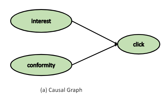
相应的causal model为: \[ S_{\mathrm{ui}}=S_{u i}^{\text {interest }}+S_{u i}^{\text {conformity }} \tag{1} \] 相应的SCM(structural causal model)为: \[ \begin{array}{l} X_{u i}^{i n t}:=f_{1}\left(u, i, N^{i n t}\right) \\ X_{u i}^{c o n}:=f_{2}\left(u, i, N^{c o n}\right) \\ Y_{u i}^{\text {click }}:=f_{3}\left(X_{u i}^{i n t}, X_{u i}^{c o n}, N^{\text {click }}\right) \end{array} \tag{2} \] 在这里我们引入Causal Embedding,为每个用户设计相应的interest embedding和conformity embedding;与之相对应的,为每个商品也设计对应的characteristic embedding(在这里叫做interest)和popularity embedding(在这里叫做conformity)
使用Causal Embedding将SCM细化得到: \[ \begin{array}{l} s_{u i}^{i n t}=\left\langle u^{(\text {int })}, i^{(\text {int })}\right\rangle , \\ s_{u i}^{c o n}=\left\langle u^{(\text {con })}, i^{(\text {con })}\right\rangle , \\ s_{u i}^{\text {click }}=s_{u i}^{i n t}+s_{u i}^{c o n} , \end{array} \tag{3} \]
Disentangled Representation Learning
我们将训练数据根据不同的causes(user’s interest,user’s conformity)分为不同的cause-specific parts,为每种原因训练不同的embedding。
但是根据数据集,我们只能知道用户是否点击了某个商品,无法知道是因为具体哪个cause而进行点击的。为了获得cause-specific的训练数据,我们引入了colliding effect这个概念!
colliding effect :
In fact, the two causes of a collider are independent variables. However, if we condition on the collider, the two causes become correlated with each other, and we call it colliding effect.
根据这一概念我们将采样两类数据(其中\(M^{I}\), \(M^{C}\)均是\(\mathbb{R}^{M \times N}\)类型的矩阵,分别表示interest matching score和conformity matching score):
Case 1: 负样本的流行性低于正样本 \[ \begin{array}{l} M_{u a}^{C}>M_{u b}^{C} \\ M_{u a}^{I}+M_{u a}^{C}>M_{u b}^{I}+M_{u b}^{C} \end{array} \tag{4} \]
Case 2: 负样本的流行性高于正样本 \[ \begin{array}{l} M_{u c}^{I}>M_{u d}^{I} \\ M_{u c}^{C}<M_{u d}^{C} \\ M_{u c}^{I}+M_{u c}^{C}>M_{u d}^{I}+M_{u d}^{C} \end{array} \tag{5} \]
首先我们组装training instance为一个三元组 (u,i,j) 即一个正样本对应特定个数个负样本()。将所有的training instance的集合称为\(O\),然后根据以上两个Case,将\(O\)分为\(O_{1}\) 和 \(O_{2}\)
接下来,将采取结合矩阵分解和BPR Loss的方法来建模以上的不等式关系,借此来学习矩阵\(M^{I}\), \(M^{C}\)。我们将整个学习过程化为四个步骤:
Conformity Modeling:
用于通过BPR Loss建模公式(4),(5)中的关于conformity的不等式关系
\[ \begin{aligned} L_{\text {conformity }}^{O_{1}} &=\sum_{(u, i, j) \in O_{1}} \operatorname{BPR}\left(\left\langle\boldsymbol{u}^{(\text {con })}, \boldsymbol{i}^{(\text {con })}\right\rangle,\left\langle\boldsymbol{u}^{(\text {con })}, \boldsymbol{j}^{(\text {con })}\right\rangle\right), \\ L_{\text {conformity }}^{O_{2}} &=\sum_{(u, i, j) \in O_{2}}-\mathrm{BPR}\left(\left\langle\boldsymbol{u}^{(\mathrm{con})}, \boldsymbol{i}^{(\mathrm{con})}\right\rangle,\left\langle\boldsymbol{u}^{(\mathrm{con})}, \boldsymbol{j}^{(\mathrm{con})}\right\rangle\right), \\ L_{\text {conformity }}^{O_{1}+O_{2}} &=L_{\text {conformity }}^{O_{1}}+{L}_{\text {conformity }}^{O_{2}} . \end{aligned} \tag{6} \]
Interest Modeling:
用于通过BPR Loss建模公式(5)中的关于interest的不等式关系
\[ L_{\text {interest }}^{O_{2}}=\sum_{(u, i, j) \in O_{2}} \operatorname{BPR}\left(\left\langle u^{(\text {int })}, i^{(\text {int })}\right\rangle,\left\langle u^{(\text {int })}, j^{(\text {int })}\right\rangle\right) \tag{7} \]
Estimating Clicks:
用于通过BPR Loss建模公式(4),(5)中的关于最终点击率的不等式关系
\[ L_{\text {click }}^{O_{1}+O_{2}}=\sum_{(u, i, j) \in O} \operatorname{BPR}\left(\left\langle\boldsymbol{u}^{t}, \boldsymbol{i}^{t}\right\rangle,\left\langle\boldsymbol{u}^{t}, \boldsymbol{j}^{t}\right\rangle\right) \tag{8} \] 其中\(\boldsymbol{u}^{t}, \boldsymbol{i}^{t}\) 和 \(\boldsymbol{j}^{t}\)分别表示为: \[ \boldsymbol{u}^{t}=\boldsymbol{u}^{(\mathrm{int})}\left\|\boldsymbol{u}^{(\mathrm{con})}, \boldsymbol{i}^{t}=\boldsymbol{i}^{(\mathrm{int})}\right\| \boldsymbol{i}^{(\mathrm{con})}, \boldsymbol{j}^{t}=\boldsymbol{j}^{(\mathrm{int})} \| \boldsymbol{j}^{(\mathrm{con})} \tag{9} \]
Discrepancy Task:
目标是使得同一user/item之间的interest embedding和conformity embedding之间的区别加大,减小两者间共同包含的信息
这里我们使用:distance correlation (dCor)来增强相应embedding之间的距离
Multi-task Curriculum Learning
多任务学习:把多个相关(related)的任务放在一起学习,同时学习多个任务。
课程学习策略:进行从易到难的学习。
对之前分解的四个子任务进行多任务学习,总的Loss为: \[
L=L_{\text {click }}{\mathrm{O}_{1}+\mathrm{O}_{2}}+\alpha\left(L_{\text {interest }}{\mathrm{O}_{2}}+{L}_{\text {conformity }}{\mathrm{O}_{1}+\mathrm{O}_{2}}\right)+\beta L_{\text {discrepancy }} \tag{10}
\] 对于之前的training instance的组装,我们采用特殊的负采样方式,即Popularity based Negative Sampling with Margin (PNSM),即:
If the popularity of the positive sample is p, then we will sample negative instances from items with popularity larger than p + mup, or lower than p − mdown , where mup and mdown are positive margin values.
这里我们通过动态调整超参数来实现课程学习策略,为了让模型的学习变得由易到难,整个过程展示如下:
- 先让模型进行简单学习,即将mup and mdown 设置的较大,使得正样本和负样本之间有很大的区分,使模型去学习具有高可信度的样例,同时将\(\alpha\)的值设置较大
- 随后逐渐增加难度,即按照0.9的比率对mup,mdown和\(\alpha\)进行衰退
数据集构造
- 为了构造和训练集I.I.D.不相同的测试集,我们按照流行性的倒数对测试集中的交互记录进行抽样
(DICE) Disentangling User Interest and Conformity for Recommendation with Causal Embedding 论文阅读