推荐系统的评测标准

hit@k

定义如下：

In a nutshell, it is the count of how many positive triples are ranked in the top-n positions against a bunch of synthetic negatives.

具体计算方法为：

In the following example, pretend the test set includes two ground truth positive only:

Jack   born_in   Italy
Jack   friend_with   Thomas

Let's assume such positive triples (identified by * below) are ranked against four synthetic negatives each. Now, assign a score to each of the positives and its synthetic negatives using your pre-trained embedding model. Then, sort the triples in descending order. In the example below, the first triple ranks 2nd, and the other triple ranks first (against their respective synthetic negatives):

s        p         o            score   rank
Jack   born_in   Ireland        0.789      1
Jack   born_in   Italy          0.753      2  *
Jack   born_in   Germany        0.695      3
Jack   born_in   China          0.456      4
Jack   born_in   Thomas         0.234      5

s        p         o            score   rank
Jack   friend_with   Thomas     0.901      1  *
Jack   friend_with   China      0.345      2
Jack   friend_with   Italy      0.293      3
Jack   friend_with   Ireland    0.201      4
Jack   friend_with   Germany    0.156      5

Then, count how many positives occur in the top-1 or top-3 positions, and divide by the number of triples in the test set (which in this example includes 2 triples):

Hits@3= 2/2 = 1.0
Hits@1= 1/2 = 0.5

对于Rank-Aware Evaluation Metrics我们一般分为两类，即 binary relevance based metrics （MRR、MAP、AUC）和 utility based metrics （NDCG）。基于排序的指标一般均为位置敏感评价指标。

位置敏感评价指标：正确推荐的item在列表中越靠前，其贡献的推荐效果越大，反之，正确推荐的item在列表中越靠后，贡献的推荐效果越小。

MRR

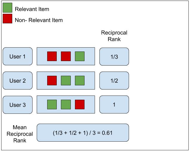
找出该query相关性最强的文档所在位置，并对其取倒数，即这个query的MRR值。对所有query的MRR值取平均即可得到该数据集上的MRR指标，显然MRR越接近1模型效果越好。但该指标的缺陷在于仅仅考虑了相关性最强的文档所在的位置带来的损失。

具体公式如下： \[ \mathrm{MRR}=\frac{1}{|Q|} \sum_{i=1}^{|Q|} \frac{1}{\operatorname{rank}_{i}} \]

优点

1. 简单易算
2. 用于计算最适合的item的情况

缺点

1. 只考虑了第一个命中的item，没有考虑其余的item
2. 不适用于比较不同的推荐序列之间的优异程度

MAP

首先为了定义MAP需要确定一个参数k，k代表前k个documents。接下来定义 P@k ： \[ P @ k(\pi, l)=\frac{\left.\sum_{t \leq k} I_{\left\{l_{\pi}-1(t)=1\right.}\right\}}{k} \] 这里 \(\pi\) 代表documents list，即推送结果列。 \(\boldsymbol{I}\) 是指示函数， \(\pi^{-1}(t)\)代表排在位置 \(t\) 处的document的标签（相关为1，否则为0）。这一项可以理解为前k个documents中，标签为1的documents个数与k的比值。

再定义Average Precision(AP) ： \[ \mathrm{AP}(\pi, l)=\frac{\left.\sum_{k=1}^{m} P @ k \cdot I_{\left\{l_{\pi}-1_{(k)}=1\right.}\right\}}{m_{1}} \] 其中 代表与该query相关的document的数量（即真实标签为1）， 则代表模型找出的前 个documents。

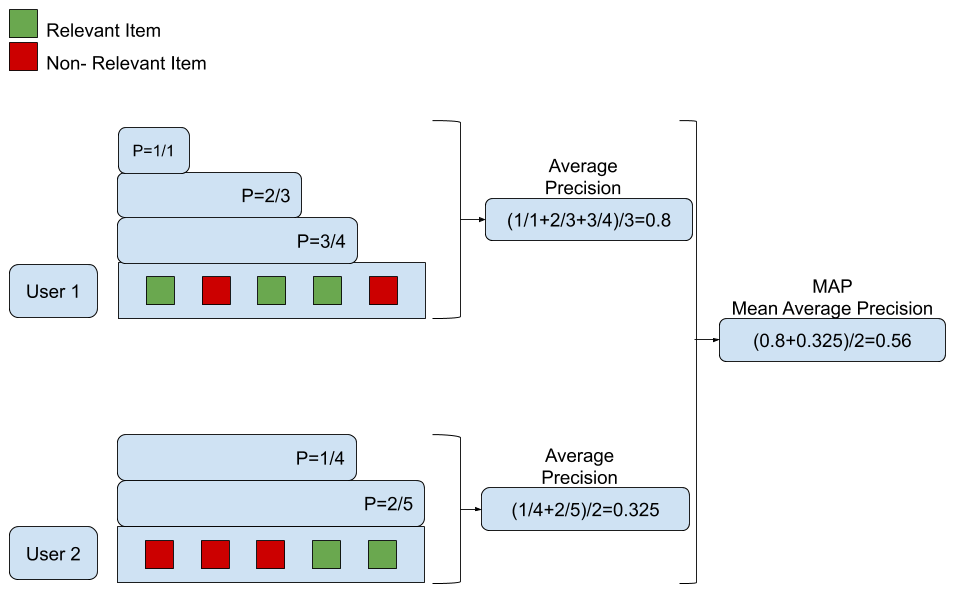
得出该query的AP值以后，MAP 值就是把所有query的AP值都计算出来再取平均即可。具体计算方式可见下图：

优点

1. 给与排在前的推荐错误的item更大的惩罚；给排在后的推荐错误的item较小的惩罚
2. 可用于比较推荐序列的排序问题

缺点

1. 只用于二进制评级（相关/不相关），不适合于基于评分的评级（1星到5星）——即细粒度的评分

NDCG@k

全名Normalized Discounted Cumulative Gain，是一个测量排序质量的指标。我们将会分成三个步骤来介绍，即：

1. Cumulative Gain(CG)
2. Discounted Cumulative Gain(DCG)
3. Normalized Discounted Cumulative Gain(NDCG)

CG

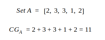
每一个待推荐的item都有一个相关性的得分，所有相关性得分总和即为CG，对于推荐系统给出的已排序（按照推荐算法）序列A，其中相关性得分（与推荐系统的推荐顺序无关）和CG分别如下所示：

DCG

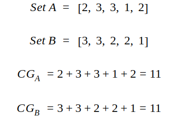
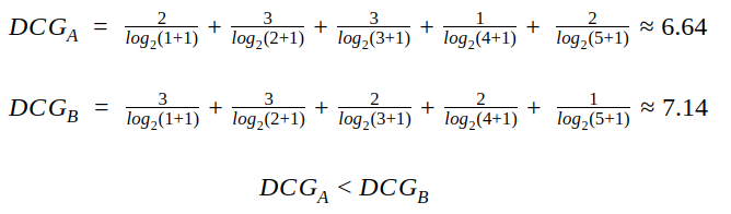
对于推荐系统给出的两个有序推荐序列A和B，虽然B的结果比A的要好（按相关性从大到小进行排序），但是按照CG进行评测两者表现效果相同，因此单纯依靠CG存在很大的缺陷

因此我们提出DCG，希望能够测量推荐系统能否将待推荐的item按照相关性的降序进行排列，其公式如下： \[ DCG=\sum_{i=1}^{n} \frac{2^{r e l e v a n c e_{i}}-1}{\log _{2}(i+1)} \] 或者 \[ DCG=\sum_{i=1}^{n} \frac{\text {relevance}_{i}}{\log _{2}(i+1)} \]

其中第一个公式对于具有较高相关性但在推荐序列中排名较后的item具有很大的惩罚，可以作为对于推荐系统排序能力进行测量的工具。对于前面举例子的集合A，B，其DCG的得分如下：

如果相关性用0/1来表示，则两个公式的效果相同

NDCG

由于不同推荐系统对于不同用户给出的待推荐序列的长度不同，相关度的范围不同，因此DCG无法作为一个通用的衡量标准，为了使其通用化，我们引入了NDCG，对于每一个推荐系统生成的序列，其计算方法如下：

1. 按照推荐系统给出的顺序计算DCG
2. 按照相关性排序的顺序计算DCG，带到iDCG
3. 求出两者的比率DCG/iDCG，取值范围应该在0,1之间

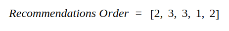
举例如下，对于推荐系统给出的序列：

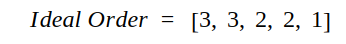
按照相关性排序可以得到：

两个序列DCG分别计算如下：

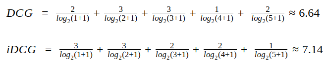
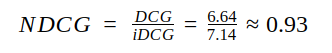
因此该序列NDCG为：

优点

1. 考虑了分级相关性值
2. 相比于MAP，NDCG在考虑推荐序列中每个元素间的先后顺序中表现的更好

缺点

1. iDCG存在等于0的情况
2. NDCG@K被提出应用于top-k排序的问题，但是存在返回结果小于k的情况，此时，我们可以用最小的得分进行padding

Reference

[1] How is hits@k calculated and what does it mean in the context of link prediction in knowledge bases

[2] Evaluate your Recommendation Engine using NDCG

[3] Learning to Rank读书笔记--排序评价指标

[4] MRR vs MAP vs NDCG: Rank-Aware Evaluation Metrics And When To Use Them